Finding better VAD parameters

A few years ago, I created a library for running a voice activity detection model in the browser. The library was intended to make it easy to create web experiences where you need to prompt the user for mic permissions, start recording audio, and work with a stream of events like “speech started,” “speech stopped,” etc, as you may want to do when developing, say, a web-based medical scribe.

I’ve occasionally considered the problem of setting the “hyperparameters” in the VAD algorithm. The voice activity detection model itself is a neural network with parameters optimized by gradient descent, but the network’s output (a stream of predicted probabilities that each short frame of audio contains speech) is turned into the “speech started” / “speech stopped” event stream via an additional algorithm. This higher level algorithm can be tweaked by setting various parameters, the most interesting of which are:

• positiveSpeechThreshold: How high does a neural network output have to be for us to interpret it as saying “yes there is speech in this audio frame”?
• redemptionMs: Suppose the neural network suddenly changes from estimating high probabilities to low probabilities of speech in a series of audio frames. How long should we wait before producing the “speech stopped” event?
• minSpeechMs: What is the minimum allowed duration of a speech segment? Any segment shorter than this will be thrown out.

These parameters tweak the behavior of the VAD in interesting ways, such as:

• How aggressively do we want to identify speech? positiveSpeechThreshold plays a role in navigating this classic “precision” vs “recall” tradeoff.
• How aggressively do we want to split utterances on silence? In a conversational voice AI application, setting redemptionMs too low could cause the voice agent to respond too aggressively, interrupting the user when they were just pausing to breathe or clear their throat. On the other hand, setting it too high could increase the voice agent’s response latency to an unacceptable degree.

The optimal tradeoffs will be different in different applications. Moreover, different apps will tend to be used in different acoustic environments, creating further differences in the optimal parameter choices.

So, how can you set these three parameters in a principled way? While I’m not an expert in this technology, I thought this would be an interesting problem to explore, and a good excuse to build pretty data collection site and do some statistical modelling. And at the end, I hoped I might have some better default parameters to ship.

Models

Define $\theta = (\text{positiveSpeechThreshold}, \text{redemptionMs}, \text{minSpeechMs})$ for convenience. To choose $\theta$ in a data-driven way, we need people to observe VAD behavior under different values of $\theta$ and submit some form of feedback, and then model their feedback in a way that enables us to optimize $\theta$.

My first instinct was to create a data collection site that allows a visitor to observe the performance of the VAD under different values of $\theta$ and submit simple “thumbs up” or “thumbs down” judgements. We could assume a parametric form for the likelihood function (i.e. the probability of a thumbs up given a particular value of $\theta$, considered as a function of $\theta$) and use maximum likelihood estimation to select $\theta$. As a simple example, we might assume that the likelihood function has a global optimum at some point $\theta_0$ and decreases as $\theta$ gets further from $\theta_0$ according to the following form:

However, after some back and forth with Claude, I settled on a different approach. The data collection site that I built (well, that Claude built) allows the user to try out the VAD, observing its behavior under two different values of $\theta$ simultaneously. At the end of recording, the user submits two pieces of feedback:

1. They highlight the regions in the audio timeline that they would have wanted the VAD to emit.
2. They decide which parameter set they liked more overall.

For a single session where a user goes through this process, we get the following data:

1. The two $\theta$ values that were compared.
2. The “probability trace,” i.e. an array containing the VAD model’s estimated probability for each audio frame during the session.
3. The user’s annotated ideal regions, i.e. where they marked that they would have liked to see the VAD emit audio.
4. The user’s choice of which of the two parameter values performed better.

Instead of modeling the likelihood function of $\theta$ directly, we instead model user preference as a function of different types of error:

1. $x^{\text{missed}}(\theta)$ is the false negative rate, in milliseconds per minute, of audio emitted by the VAD when using settings $\theta$. For a given session, we can compute it by calculating the duration of audio in the user’s annotated ideal regions that does not appear in the audio emitted by the VAD, and then dividing by the duration of the session.
2. $x^{\text{excess}}(\theta)$ is the false positive rate, in milliseconds per minute, of audio emitted by the VAD when using settings $\theta$. For a given session, we can compute it by calculating the duration of audio emitted by the VAD that does not appear in the user’s annotated ideal regions.

Suppose a user’s overall utility when using the VAD is a weighted sum of these two errors:

We can interpret $p$ as saying that one millisecond of speech lost is worth $p/(1-p)$ milliseconds of stray audio. We can model the process of the user visiting the data collection site as them making a noisy observation of the two utilities and choosing the option with the higher observed value. If we assume, for convenience and tradition, that the noisy observations can be modeled as

where $\varepsilon_A$ and $\varepsilon_B$ are IID random variables following a Gumbel distribution, then we can infer that

where

• $\beta = (p, 1-p) = (\beta^{\text{missed}}, \beta^{\text{excess}})$ is vector notation for the unknown error weights, useful for conciseness and in case we want to add new types of errors later on.
• $x(\theta) = (x^{\text{missed}}(\theta), x^{\text{excess}}(\theta))$ is vector notation for the observed error values.
• $\sigma$ is the distribution function of the logistic distribution.
• $\lambda$ is a scale parameter for the logistic distribution, representing the unknown degree of noisiness in the utility observations.
• $\langle\cdot,\cdot\rangle$ is simply notation for the dot product.

It turns out that we stumbled into something called discrete choice analysis.

Now we have a foundation for optimizing $\theta$, which looks like this:

1. Estimate the parameters $\beta$ and $\lambda$ using the observed choices and error $(\text{i.e. }x(\theta))$ values collected from the site, thereby giving us an estimated utility function.
2. Recall that we are also collecting probability traces and annotated ideal regions. That means that for any $\theta$ (not just the values observed and compared by the user), we can “replay” the algorithm that parses probability traces into “speech start” / “speech stop” events. In other words, we can use the annotated ideal regions to compute the error vector $x(\theta)$ for any $\theta$ for any probability trace we collected. Therefore, we select $\theta$ by searching $\theta$-space for the value that maximizes the expected value of the estimated utility function.

Why would we prefer this to the first model I outlined above, where I specified the likelihood of a “thumbs up” in terms of $\theta$? The benefits, to my mind, are that

1. I feel more confident that user preference is driven by errors like “missing” and “excess” audio than I do in specifying a particular parametric form for the likelihood of $\theta$. Misspecifying the likelihood (e.g. getting the shape or functional form wrong) could bias the $\theta$ estimate. In this way, decomposing the problem into the preference model and a search in $\theta$-space captures my intuitions about the problem better and forces me to make fewer arbitrary modeling decisions.
2. Instructing users to mark which of two VADs they liked more seems less error-prone/ambiguous than instructing them to observe one single VAD and give a thumbs up/thumbs down judgement. A concrete comparison is less subjective and potentially carries more information about what kinds of errors actually matter.

That being said, these are loosely held opinions – I could be wrong in thinking that this is the better approach. If my interest here was more than recreational, I would try to implement a better workflow, fit multiple models, etc.

Results

After having Claude create the data collection site, I did a few sessions to gather data. I spent very little time on this – just 6 sessions amounting to ~2 min of recorded audio – and wasn’t expecting much in the way of results. As it turns, out, though, even this small amount of data turned out to be fairly informative.

After observing two $\theta$ values in each of six sessions, I had 12 points $x(\theta)$ in the two-dimensional error space. Coloring each point according to whether it was the $\theta$ I marked as “preferred” during its session produces the following plot (with arrows drawn from the dis-preferred to the preferred point for the same session):

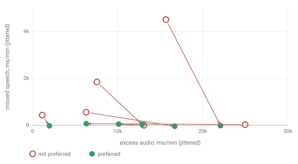
It’s clear from the plot that missed speech was more important than excess audio in that I always preferred the $\theta$ with lower missed speech. Moreover, it doesn’t seem that difficult to find $\theta$ values that don’t miss speech – even my dumb $\theta$ sampling mechanism got no missed speech around half the time. Finally, in the cases where both $\theta$s being compared did not miss any speech, I preferred the $\theta$ with lower excess audio.

What kind of error rates does the current $\theta$ that I’m shipping in the library get? Here is the plot above but with the error values for the default $\theta$ added in:

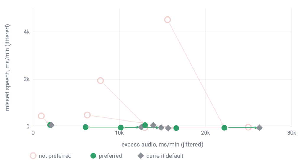
The current default $\theta$ does well on capturing all speech, but it scores worse on excess audio than almost all of the $\theta$ values generated during data collection. Let’s see if we can find a new $\theta$ that does better.

To estimate $\beta = (p, 1-p)$, I set a couple of different priors on $p$ and calculated the posterior mean. For brevity, I’ll just mention the results when using a uniform prior on the unit interval for $p$, which leads to results similar to other priors and sufficiently motivates the rest of the analysis. The uniform prior produces a posterior mean of 0.939 and a credible interval of 0.823-0.993. In other words, each millisecond of missed speech is worth about $0.939/(1-0.939)=15.4$ milliseconds of excess speech.

The next step is to plug the estimated $\beta$ in to the utility formula and search for a $\theta$ that maximizes it. It turns out that utility keeps increasing as positiveSpeechThreshold increases even into values as high as 0.99. However, I did not sample any values of positiveSpeechThreshold higher than 0.8, and I suspect that my audio setup was better than most (which might mean that higher speech thresholds work better in my setup than for others). So, I’m hesitant to accept the model’s implication that values of positiveSpeechThreshold as high as 0.99 are optimal. I decided to constrain the $\theta$ search to values where positiveSpeechThreshold was at most 0.8.

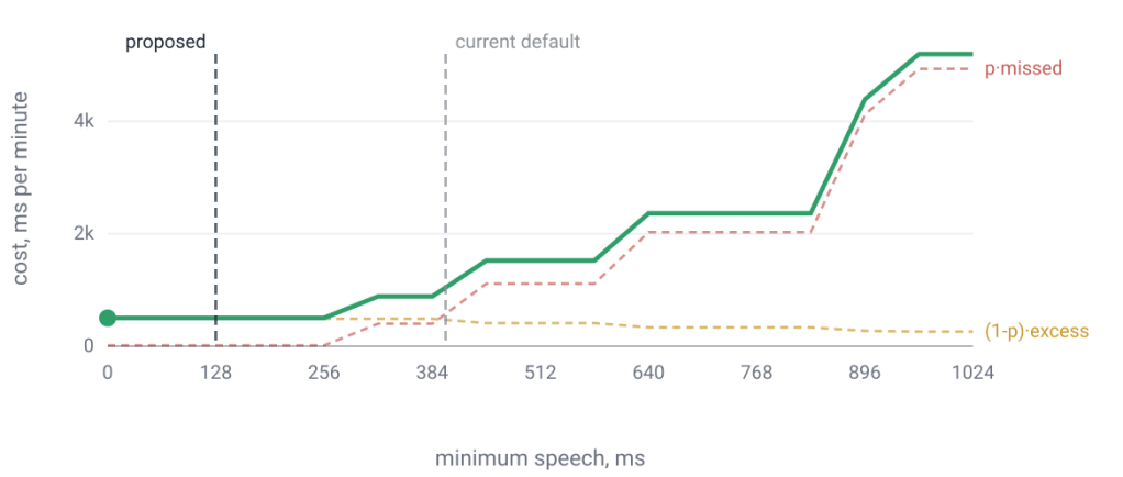
Given this constraint, utility was maximized in the region ${0.8} × {576} × [0, 256]$: positiveSpeechThreshold set to 0.8, redemptionMs set to 576, and minSpeechMs set to any value less than 256. I decided that setting minSpeechMs to 128, well in the interior of the $[0, 256]$ interval, was a reasonable choice.

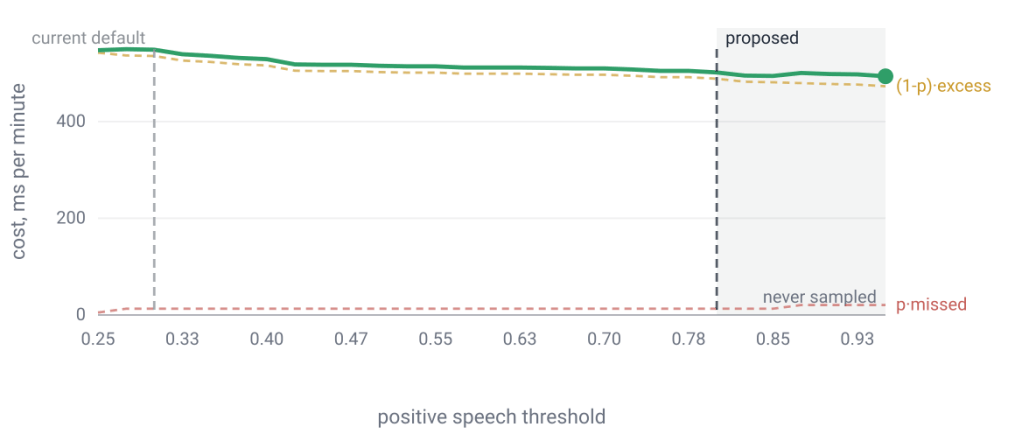
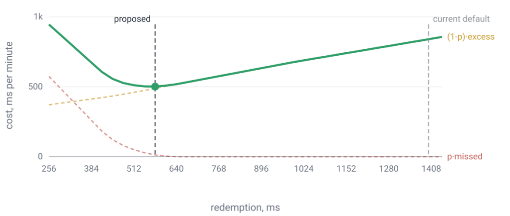
I wanted to get some sense of the shape of the utility function, so here are plots showing how utility (plotted as negative utility, or “cost,” for visual clarity) changes with each component of $\theta$, holding the other components fixed at their final estimates (the final estimates being $(0.8, 576, 128)$). You can see that the utility does not strongly discriminate between positiveSpeechThreshold values – for redemptionMs set to 576 and minSpeechMs set to 128, utility is somewhat flat but generally improves slightly (i.e. the plotted negative utility goes down) as positiveSpeechThreshold increases. This makes sense to me because the Silero VAD model is highly accurate. In most cases, when you start talking, you can see the frame-by-frame probability jump from around 0 to around 1, so it shouldn’t matter too much where in the middle you decide to set the threshold. The utility is a bit more sensitive to redemptionMs and minSpeechMs, where I think the optimized values may be noticeably better than the current defaults.

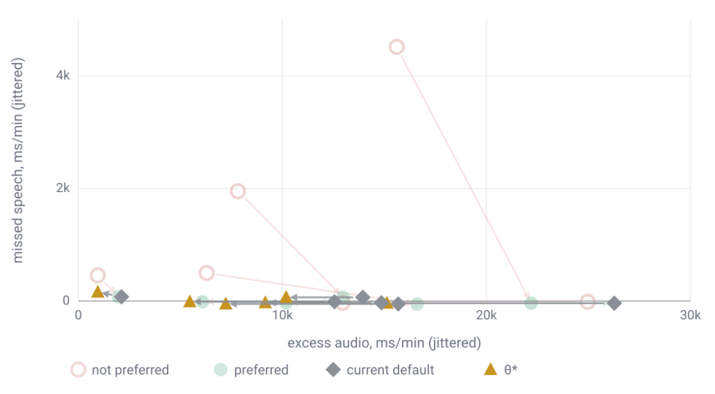
It’s a bit hard to read, but we can plot how the error changes when using this new $\theta$ instead of the defaults for the test session data:

Perhaps the directionality of the difference is more apparent with this animated plot of the test session error values against different $\theta$:

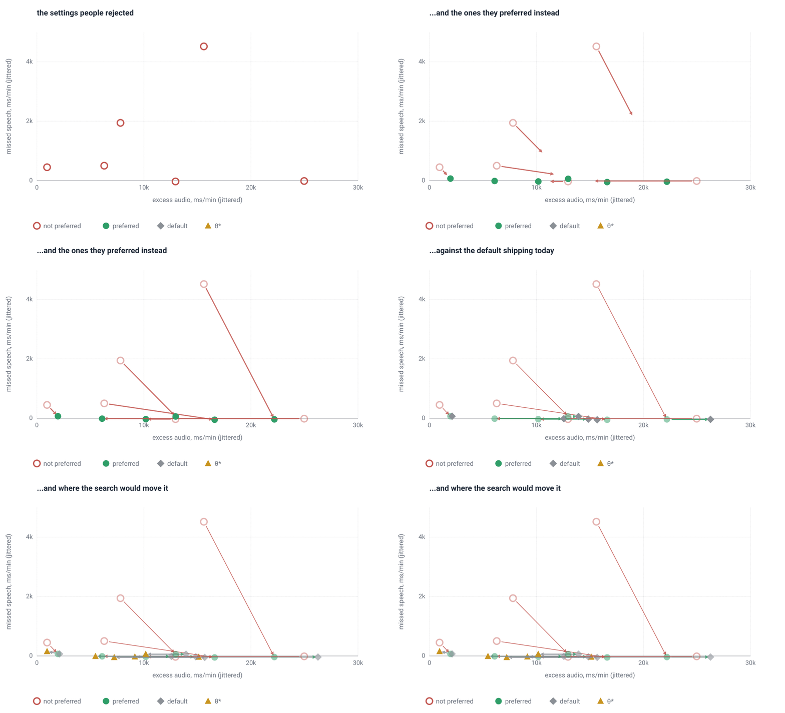
Even with this small amount of data, I feel fairly confident that this new $\theta$ is better than what I had arbitrarily set as the library default long ago.